
My data looks like this, but imagine the dates cover a full year and there are many more widget codes.
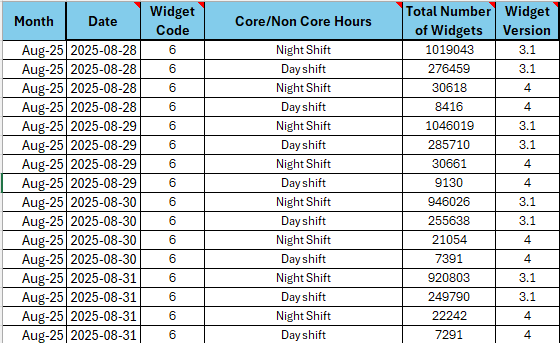
I need to determine, for a given widget code and month, the maximum number of widgets produced in a single day across the two shifts, regardless of widget version.
MAXIFS using the month and widget code as criteria won't work, cos that'll just pull back the greatest single cell and I need the maximum of the sum of the multiple rows that relate to a single day.
Ideas?
I'd use Get Data to pull that table into the data model then use Power Query to wrangle it to produce an output table of month, widget, max daily sum. That's not something I can describe step by step from my phone though!
Edit - or you can probably get away with doing it via a pivot table to give the sum of each widget by day then using maxifs on that.
Is that not a pretty simple Pivot Table?
Pivot table.
With a sum for each month and wdget.
I can't think off my head if you can combine date and widget. The usual way round the is to concatenate your two columns to create a unique singecell id =a2&b2 then set that as your pivot series.
I am post marathon today so might be talking gibberish but its something like that.
It's definitely doable in a Pivot Table, but I need the value to appear in a cell in a 'monthly summary data' tab that has various totals/stats for each month and pulls data from various places. I've been asked to add 'greatest number of each widget type produced in a single day' to that tab, and that needs to auto-populate/calculate for each month from the source data (which is the table above).
You can have more than one pivot table. Have a sheet with all the pivot tables arranged like a dashboard. Or take the answers somewhere else. If you already have a sheet in mind.
If you wantto do ot manually then something like
=A1&A2
Then use an UNIQUE or some INDEX(thats an array formula so needs to be entered correctly ) to build a list of all the above combinations (a single row for each combo)
Then on the next columns use lookups and sums and maximums to build the table you want.
That will give you a dynamic list of date and widget values.
Did it - used SUMIFS as an array formula with
- the month and widget codes as criteria
- an additional criteria that used SEQUENCE to create a range of all the dates in a given month
That gave an array of total volumes per day for the given month and widget, then did a MAX of that array
{MAX(SUMIFS(WidgetCount,[WidgetCode,GivenWidgetCode],[Month,GivenMonth],[Date,(SEQUENCE(DaysInMonth,1,Month StartDate,1))]))}
Easy, eh?
I was about to suggest SUMIFS but you got there on your own.
tbh, stuff like this is ChatGPT's forte. throw what youve put into it and itll sort you out:
Exactly — you’ve spotted the limitation of
MAXIFS: it works on single cells, not on grouped daily totals.✅ Goal restated:
For each Month and Widget Code, find the maximum total widgets produced in a single day — summing both Day + Night shifts (and ignoring Widget Version).
💡 Option 1: Use a Pivot Table
Select your full dataset.
Go to Insert → PivotTable.
In the PivotTable Field List:
Drag Month → Rows
Drag Widget Code → Rows (below Month)
Drag Date → Rows (below Widget Code)
Drag Total Number of Widgets → Values → change to Sum of Total Number of Widgets
Now you have total widgets per day.
To get the maximum per month & widget code:
Right-click the Pivot → Show Values As → None (to keep raw sums)
Then either:
Add another pivot on top of this one summarizing by Month + Widget Code and using Max of Total per Day, or
Copy the daily totals into a new table and use
=MAXIFS(...)on those summed values.🔸 Best for: visual exploration and flexible reporting.
💡 Option 2: Use a Helper Column + MAXIFS
Add a helper column:
=SUMIFS([Total Number of Widgets],[Date],[@Date],[Widget Code],[@[Widget Code]])
→ This gives the total widgets per widget code per date.
(If you have multiple months, includeMonthas a criterion.)Then use:
=MAXIFS([HelperColumn],[Month],targetMonth,[Widget Code],targetCode)🔸 Best for: staying purely formula-based without pivots.