![]() You don't need to be an 'investor' to invest in Singletrack: 6 days left: 95% of target - Find out more
You don't need to be an 'investor' to invest in Singletrack: 6 days left: 95% of target - Find out more
Okay Excel ninjas here goes:
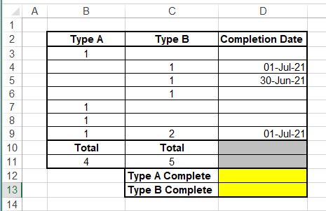
What I'm trying to achieve is totalling all of the Completed Type As in cell D12 and Completed Type Bs in D13.
A bit of Googling has taken me to the COUNTIFS function but I'm not sure if its suitable for this particular conundrum.
Ta in advance.
https://exceljet.net/formula/sum-entire-column
Would this work ?
Sorry, ignore didn't read it properly, will have a think
in D12 = SUMIF (D3:D9, ">0", B3:B9)
*Edit - simplified it
Yeah, countifs will work for that
=COUNTIFS(b3:b9,1,D3:D9,">0")
I'm with t' purist on this: sumif.
How will countif work for the brace in C9?
Type A Complete : =SUMIF(D3:D9,"<>",B3:B9)
Type B Complete : =SUMIF(D3:D9,"<>",C3:C9)

Cheers all. I'll give that a try on Monday.
(And yes, we are pretty much off of the right hand side of that graph up there ^^)
=SUM(IF(D3:D9>0,B3:B9,0)
Simple array formula.
That will go down column D and where the entry is greater than 0 (i.e. a date value is present) it will add in the corresponding B column value on the same line, if column D is blank/not greater than 0 then it will return a zero within the SUM.
You might need ctrl+shift+enter rather than just enter depending on your excel version.
SUMIF above is also good but I find this array format a bit more flexible (I think for example that SUMIF will only work vertically which is fine here but may not be on a different issue later).
I find sumproduct great for this sort of stuff…
In D12:
=SUMPRODUCT((D3:D9>0)*(B3:B9>0))
For d13 change b3:b9 to c3:c9
(I’ll mock it up in excel when I’m next on my pc to make sure I have the syntax right!)
Ditto the sumif answers as you're looking for the total if more than one criteria are met.
Party pooper...prepared to be laughed at...but wouldn't it be easier just to have 2 columns for completion date..
One for type A next to type A count and one next to type B...looks to me that unless you are safely pulling the count data in then someone could enter Type A count and Type B count and a date that may apply to either all on the same line potential for the not unusual "I don't know it wasn't my spreadsheet but it told me to do it"
Two columns only would make sense then you could do something like COUNT and whatever the non blank formula is. You could VBA it to create a popup if someone enters dates in both cells by mistake.
Edit: COUNTA
Just checked the SUMPRODUCT solution I posted above, it should be...
=SUMPRODUCT((D3:D9>0)*B3:B9)
=SUMPRODUCT((D3:D9>0)*C3:C9)